Are nonsensical models useful?

27 April 2018 - 7 mins read time
Tags: Statistics

One of the first principles that I ever learned about creating mathematical models was this:

“Models must not predict absurdities.”¹

A further explanation in the original text is that absurd models are a common pitfall in social sciences and physicists would refine models until they conform to even extreme cases.

I’ve always taken that principle literally. But models often do predict absurdities. This is commonplace with linear regeression models and even in academic reseach. Simple linear regression models often predict a theoreticaly impossible situation where response is 0 while the value of predictor is not. Nevertheless, coercing the intercept to 0 (regression through the origin) is usually strongly argued against. So there is a conflict between what theory and methodology suggest. How is this possible? I argue that the problem stems from the fact that we too often assume relationships to be linear (even with untransformed and unnormalized data), while this is almost never the case outside hard sciences.

I tend to think visually, so this is how I’ll try to explain this dilemma. First off, because we’ll need to repeat the visualization of the same data for different models, let’s create a few functions for the sake of concision.

# Define a function to plot points from women dataset
plotData <- function() {
  plot(c(0,75), c(0,200), type = 'n', xlab = "Height (in)", ylab = "Weight (lb)")
  points(women)
}

# Define a function to add model fit to a plot
addFit <- function() {
  predicted <- predict(model, data.frame(height = 0:200), type = 'response')
  lines(0:200, predicted, col = 'cornflowerblue')
}

We’ll use the women dataset that comes with base R to predict weight from height. Probably the simplest solution to this problem is a simple linear regression estimation.

(model <- lm(weight ~ height, women))

## 
## Call:
## lm(formula = weight ~ height, data = women)
## 
## Coefficients:
## (Intercept)       height  
##      -87.52         3.45

plotData(); addFit()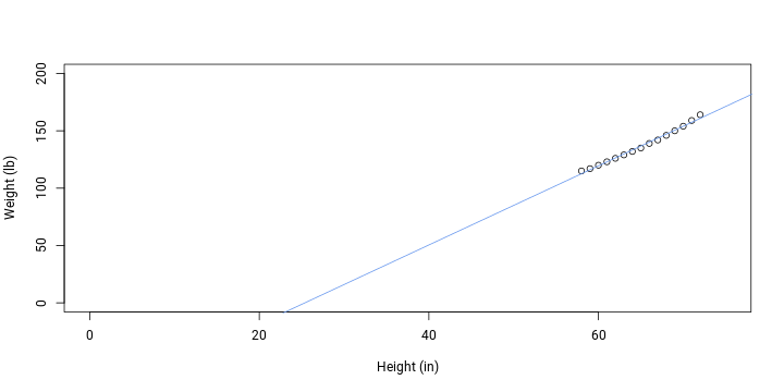

When being picky, we could say that the fit does not satisfy the normality assumption and residuals are higher at more extreme values. However, with an R-squared value of 0.991 the model captures the relationship very well.

Despite a good fit to actual data, the previous model would predict thoretically impossible value at intercept: weight is 0 lbs only until height is -88 in. Even when height is 20 in, weight is predicted to be -19 lbs. To make sure that the intercept is 0, we can drop it.

(model <- lm(weight ~ 0 + height, women))

## 
## Call:
## lm(formula = weight ~ 0 + height, data = women)
## 
## Coefficients:
## height  
##   2.11

plotData(); addFit()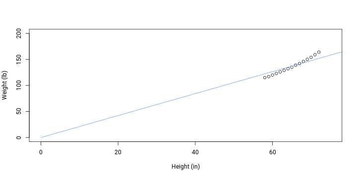

While theoretically accurate regarding intercept, a linear fit without intercept does not fit data very well. To solve this, let’s allow a curvature in the relationship by fitting a polynomial (the model will still be linear in terms of parameters).

(model <- lm(weight ~ poly(height, 2, raw = T), women))

## 
## Call:
## lm(formula = weight ~ poly(height, 2, raw = T), data = women)
## 
## Coefficients:
##               (Intercept)  poly(height, 2, raw = T)1  
##                 261.87818                   -7.34832  
## poly(height, 2, raw = T)2  
##                   0.08306

plotData(); addFit()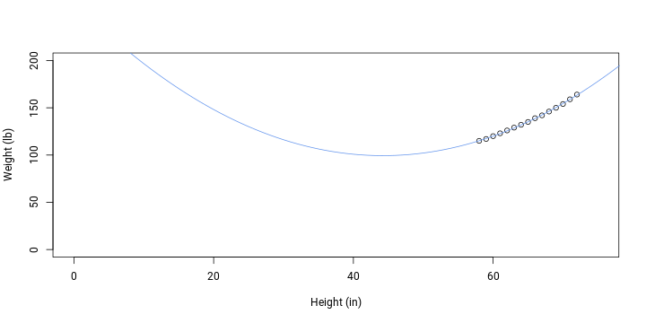

Visually, fit do data is better compared to the first model but outside data points it now makes even less sense. We can again constrain the intercept to 0.

(model <- lm(weight ~ 0 + poly(height, 2, raw = T), women))

## 
## Call:
## lm(formula = weight ~ 0 + poly(height, 2, raw = T), data = women)
## 
## Coefficients:
## poly(height, 2, raw = T)1  poly(height, 2, raw = T)2  
##                   0.73085                    0.02103

plotData(); addFit()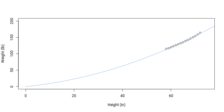

The model now fits both the theoretical assumption of 0 intercept and also data to some degree. A better result can be attained by using a 3rd degree polynomial since we wish to coerce the fit to intercept as well as data.

(model <- lm(weight ~ 0 + poly(height, 3, raw = T), women))

## 
## Call:
## lm(formula = weight ~ 0 + poly(height, 3, raw = T), data = women)
## 
## Coefficients:
## poly(height, 3, raw = T)1  poly(height, 3, raw = T)2  
##                 4.8487293                 -0.1057881  
## poly(height, 3, raw = T)3  
##                 0.0009721

plotData(); addFit()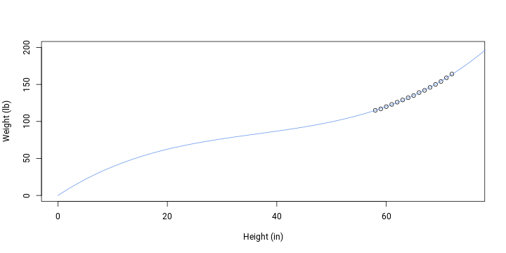

The model could further be improved not to allow weights and heights below 0. But when we only aim for a model that has an intercept of 0 (i.e. no intercept) and fits available data, the optimal formula would be this:

Weight = 4.8487 * height + -0.1058 * height^2 + 0.001 * height^3

It should now be obvious where the problem originates from. The true relationship is not linear. A model without a constrained intercept only mimics the true relationship and this is good enough only in the actually observed range of predictor values. As the value of predictor decreases, the model loses its theoretical fit. That’s why models can be reasonable while theoretically invalid. They’re only reasonable in a certain range which is all we usually need.

As demonstrated, we can correct an invalid intercept by fitting a curve instead of a straight line. But was it worth it? I don’t think so. The first and simplest model already had an excellent fit to data so we didn’t gain much in terms of explaining the relationship. Also, the concept of simple linear regression is fairly simple but the calculation of 3rd degree polynomials is not so much.

Coming back to the opening idea, I would say that models can predict absurdities but only outside real, observed values.

References