Evaluating keyboard layouts with R
The now standard Qwerty keyboard layout that originates from 19th century is often assumed to be suboptimal, reason being that it was designed to cope with mechanical limits of typewriters. In order to avoid jamming of keylevers, letters often sequentially used had to be placed apart from each other, so that the levers would not interact. While true or not, various alternative layous have been proposed that are claimed to be much better optimized with typing speed and comfort in mind. First of these was the Dvorak Simplified Keyboard (or commonly just Dvorak) in 1932 that put more emphasis on using the middle (home) row and alternating hands after each key press. This is until today the most prominent alternative layout, but Colemak designed in 2006 is becoming increasingly popular. Supposedly, Colemak further increases the use of home row, optimizes the placement of more frequent letters and improves on rolling motions. While it’s not known how exactly was the development of Colemak aided by computers, the intricate computer assisted design of Qgmlwy is publicly available on the Carpalx project website. Qgmlwy should require the least effort when typing.
This post will evaluate differet aspects of the aforementioned keyboard layouts for typing in English. The differences between these layous are known but this post will also attempt to outline the magnitudes of these differences.
Data entry
Let’s load necessary packages and objects. The latter includes theme and color scheme for plots and some functions for text formatting.
# Load packages
library('dplyr'); library('tidyr'); library('ggplot2'); library('extrafont')
# Load objects
load('data/objects/lil_theme.Rda'); load('data/objects/funs.Rda')
To begin with, we need to imput some data. American National Corpus data gives us the most common words and their relative frequencies in English. These frequencies are used as the basis for creating a text sample of 100 000 words which will be employed later in the analysis.
# Import word frequencies from ANC
en <- read.csv('http://www.anc.org/SecondRelease/data/ANC-token-count.txt',
               header = F, sep='\t', stringsAsFactors = F, encoding = 'UTF-8')
# Remove last row that indicates the word count
en <- head(en, -1)
# Change row names
names(en) <- c('word', 'count', 'freq')
# Fix words with encoding problems
en$word <- iconv(en$word, 'UTF-8', 'UTF-8', sub = '')
# Create a word sample "weighted" with frequencies
word.sample <- sample(rep(en$word, en$count), 1e+5)

SampleRows(en, 10)
## word count freq
## 26915 unsavory 31 1.398602e-06
## 185176 codefi-nitional 1 4.511621e-08
## 68544 daya 5 2.255810e-07
## 197352 kerouacian 1 4.511621e-08
## 88590 fluid-filled 3 1.353486e-07
## 115227 glutathione-coupled 2 9.023241e-08
## 225198 non-enclosed 1 4.511621e-08
## 5771 triumph 315 1.421160e-05
## 24526 mlb 36 1.624183e-06
## 156788 cunto 1 4.511621e-08head(word.sample, 10)## [1] "next" "makobane" "suggest" "in" "can" "supposed"
## [7] "yeltsin" "correct" "both" "chili"For evaluation of the placement of letters, the R’s matrix provides an appropriate data format. This does not perfectly reflect the staggered layout of most keyboards, but for the purposes here it’s close enough.
# Qwerty layout
qwe <- matrix(c('q', 'w', 'e', 'r', 't', 'y', 'u', 'i', 'o', 'p', '[', ']',
                'a', 's', 'd', 'f', 'g', 'h', 'j', 'k', 'l', ';', "'", NA,
                'z', 'x', 'c', 'v', 'b', 'n', 'm', ',', '.', '/', NA, NA),
              ncol = 12, byrow = T)
# Dvorak layout
dvo <- matrix(c("'", ',', '.', 'p', 'y', 'f', 'g', 'c', 'r', 'l', '?', '=',
                'a', 'o', 'e', 'u', 'i', 'd', 'h', 't', 'n', 's', '-', NA,
                ';', 'q', 'j', 'k', 'x', 'b', 'm', 'w', 'v', 'z', NA, NA),
              ncol = 12, byrow = T)
# Colemak layout
clm <- matrix(c('q', 'w', 'f', 'p', 'g', 'j', 'l', 'u', 'y', ';', '[', ']',
                'a', 'r', 's', 't', 'd', 'h', 'n', 'e', 'i', 'o', "'", NA,
                'z', 'x', 'c', 'v', 'b', 'k', 'm', ',', '.', '/', NA, NA),
              ncol = 12, byrow = T)
# Qgmlwb layout
qgm <- matrix(c('q', 'g', 'm', 'l', 'w', 'b', 'y', 'u', 'v', ';', '[', ']',
                'd', 's', 't', 'n', 'r', 'i', 'a', 'e', 'o', 'h', "'", NA,
                'z', 'x', 'c', 'f', 'j', 'k', 'p', ',', '.', '/', NA, NA),
              ncol = 12, byrow = T)
Data preparation
We begin by creating a matrix that has a row for each word and a column for each symbol. Values of these columns indicate the count of occurrences of these symbols.
# Create data frame containing the count of occurrences of each symbol in each word
en.df <- mapply(function(x) nchar(tolower(gsub(paste0("[^", x, "]"), "", en[, 1]))),
                sort(unique(tolower(unlist(strsplit(en[, 1], ''))))))

SampleRows(en.df, 10)
## - ? ' 0 1 2 6 7 9 a b c d e f g h i j k l m n o p q r s t u v w x y
## [1,] 1 0 0 0 0 0 0 0 0 0 0 1 0 1 0 0 0 1 0 0 0 0 0 1 1 0 1 1 1 1 0 0 1 0
## [2,] 0 0 0 0 0 0 0 0 0 1 0 0 1 2 0 0 2 1 0 0 0 0 0 0 0 0 1 0 1 0 0 1 0 0
## [3,] 0 0 0 0 0 0 0 0 0 2 0 0 1 2 0 0 0 0 0 0 1 0 1 0 0 0 1 0 0 0 0 0 0 1
## [4,] 0 0 0 0 0 0 0 0 0 1 0 1 0 1 0 0 1 1 0 0 1 1 0 0 0 0 0 0 0 0 0 0 0 0
## [5,] 0 0 0 0 0 0 0 0 0 0 0 0 0 0 0 0 0 1 0 0 1 0 1 1 0 0 0 0 2 0 0 0 0 0
## [6,] 0 0 0 0 0 0 0 0 0 2 1 0 0 1 0 0 0 0 0 0 0 0 1 0 0 0 1 0 0 0 0 0 0 0
## [7,] 1 0 0 0 0 0 0 0 0 0 0 2 1 4 1 0 0 0 0 0 0 0 1 1 0 0 3 2 0 0 0 0 0 0
## [8,] 0 0 0 0 0 0 0 0 0 1 0 1 1 0 0 0 0 2 0 0 0 0 1 1 0 0 0 0 2 0 0 0 0 0
## [9,] 0 0 0 0 0 0 0 0 0 0 1 0 0 1 0 0 0 0 0 0 0 0 2 0 0 0 1 0 1 0 0 0 0 0
## [10,] 0 0 0 0 0 0 0 0 0 1 0 1 1 1 0 0 0 1 0 0 1 1 1 0 0 0 0 0 1 1 0 0 0 0
## z
## [1,] 0
## [2,] 0
## [3,] 1
## [4,] 0
## [5,] 0
## [6,] 1
## [7,] 0
## [8,] 0
## [9,] 0
## [10,] 0After simply binding the matrix with the initial data frame, we have another data frame we can use for our evaluation.
# Join previous with the original data frame
en.df <- data.frame(en, en.df)
# Remove symbols that are not letters
en.df <- en.df[, grep('^[^X]', names(en.df))]

SampleRows(en.df, 10)
## word count freq a b c d e
## 71104 aprilbot 5 2.255810e-07 1 1 0 0 0
## 13714 ressam 89 4.015342e-06 1 0 0 0 1
## 180205 red-legged 1 4.511621e-08 0 0 0 2 3
## 134140 not-terribly-big 1 4.511621e-08 0 2 0 0 1
## 238633 our-leaders-are-all-corrupt-and-stupid 1 4.511621e-08 4 0 1 3 3
## 149773 periclitari 1 4.511621e-08 1 0 1 0 1
## 149414 topiii 1 4.511621e-08 0 0 0 0 0
## 67265 a 6 2.706972e-07 1 0 0 0 0
## 116542 ellebila 2 9.023241e-08 1 1 0 0 2
## 27781 mascot 29 1.308370e-06 1 0 1 0 0
## f g h i j k l m n o p q r s t u v w x y z
## 71104 0 0 0 1 0 0 1 0 0 1 1 0 1 0 1 0 0 0 0 0 0
## 13714 0 0 0 0 0 0 0 1 0 0 0 0 1 2 0 0 0 0 0 0 0
## 180205 0 2 0 0 0 0 1 0 0 0 0 0 1 0 0 0 0 0 0 0 0
## 134140 0 1 0 2 0 0 1 0 1 1 0 0 2 0 2 0 0 0 0 1 0
## 238633 0 0 0 1 0 0 3 0 1 2 2 0 5 2 2 3 0 0 0 0 0
## 149773 0 0 0 3 0 0 1 0 0 0 1 0 2 0 1 0 0 0 0 0 0
## 149414 0 0 0 3 0 0 0 0 0 1 1 0 0 0 1 0 0 0 0 0 0
## 67265 0 0 0 0 0 0 0 0 0 0 0 0 0 0 0 0 0 0 0 0 0
## 116542 0 0 0 1 0 0 3 0 0 0 0 0 0 0 0 0 0 0 0 0 0
## 27781 0 0 0 0 0 0 0 1 0 1 0 0 0 1 1 0 0 0 0 0 0Plot functions
To present the results of our analysis in an intuitive manner, we create a PlotBar function to illustrate results in absolute values and PlotDensity function to show the distribution of values by words.
PlotBar <- function(dat, tit, var) {
  dat %>% select(-word) %>% colSums %>% t %>% data.frame %>% gather('layout', 'val') %>%
    mutate(layout = Proper(layout)) %>%
    ggplot + aes(x = reorder(layout, val), y = val/nchar(paste(word.sample, collapse = '')),
                 fill = factor(layout, levels = c("Qwerty", "Dvorak", "Colemak", "Qgmlwb"))) +
    labs(title = tit, x = "Layout", y = var, fill = "Layout",
         caption = "Source: American National Corpus second release frequency data") +
    geom_bar(stat = 'identity', width = .6) + coord_flip() +
    ylim(0, 1) +
    geom_text(aes(label=Perc(val/nchar(paste(word.sample, collapse = '')))),
              hjust=1.2, size = 4, color = clrs$mono[1], family = 'Roboto Medium') +
    scale_fill_manual(values = clrs$dark) +
    theme_min()
}
PlotDensity <- function(dat, tit, var) {
dat %>% gather('layout', 'val', 2:5) %>%
mutate(layout = Proper(layout)) %>%
ggplot + aes(x = val/nchar(word),
color = factor(layout, levels = c("Qwerty", "Dvorak", "Colemak", "Qgmlwb"))) +
labs(title = tit, x = var, y = "Word density", color = "Layout",
caption = "Source: American National Corpus second release frequency data") +
geom_density(size = .8) +
scale_color_manual(values = clrs$dark) +
theme_min()
}Frequencies of letters on different layouts
First off, lets compare the frequecy of letters in English corpus. Each letter in our data frame is multiplied by its actual count. Then we calculate the share of each letter from all letters.
# Calculate total frequencies for each letter in each word
en.ag <- data.frame(lapply(en.df[4:dim(en.df)[2]], function(x) x * en.df$count))
# Calculate the proportions for each letter
en.ag <- en.ag %>% summarise_each(funs(sum(., na.rm = T))) %>%
  gather('var', 'val') %>% mutate(val = val/sum(val))
Let’s plot the result.
ggplot(en.ag) + aes(x = reorder(toupper(var), -val), y = val) +
  labs(title = "Frequencies of letters in English",
       x = "Letter", y = "Share out of all letters",
       caption = "Source: American National Corpus second release frequency data") +
  geom_bar(stat = 'identity', fill = clrs$dark[4]) +
  theme_min()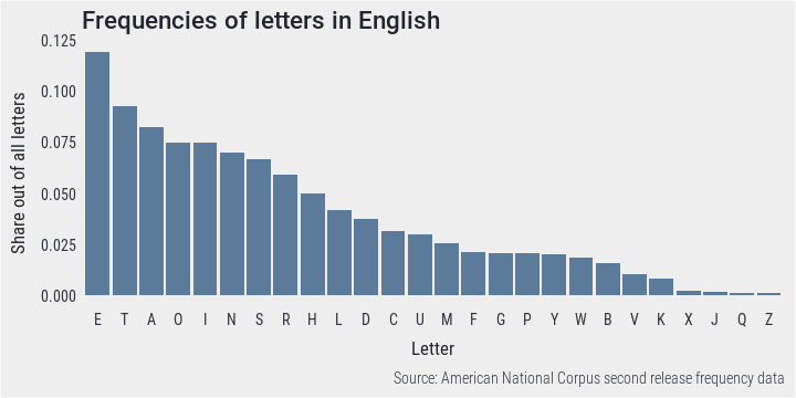
Next, we define a function PlotFreq that plots these calculated frequencies. Again, it’s not the exact impression of standard keyboards with staggered layouts but good enough. We will use this function to produce graphs for each layout
PlotFreq <- function(occurrences, layout.mat, letters, layout, color) {
  matrix(occurrences[match(layout.mat, letters)], ncol = 12) %>%
    data.frame(check.names = F) %>%
    gather(col, val) %>% group_by(col) %>% mutate(row = row_number()) %>%
    ggplot() + aes(x = factor(col, levels = 1:12),
                   y = factor(row, levels = 3:1), fill = val) +
    labs(title = paste("Frequency of letters in English on", layout, "layout"),
         fill = "Frequency on a scale from 0 to 1",
         caption = "Source: American National Corpus second release frequency data") +
    geom_raster() + coord_fixed() +
    geom_text(label = toupper(c(layout.mat)), size = 6, family = 'Roboto') +
    scale_fill_gradient(low = clrs$mono[6], high = color,
                        na.value = clrs$mono[6]) +
    theme_min()+ theme(axis.title = element_blank(), axis.text = element_blank(),
                       legend.position = 'bottom',
                       legend.key.width = unit(20, 'pt'))
  }
The placement of letters on Qwerty does imply that the layout is not optimal for touch typing. Most of the more frequent letters are on the upper row and rather infrequent letters occupy the home position of the strongest fingers. The middle row almost seems to follow the letter ordering of the alphabet. On the other hand, some more infrequent keys are on the edges which should decrease the fatigue of weaker fingers.
PlotFreq(en.ag$val, qwe, en.ag$var, "Qwerty", clrs$dark[1])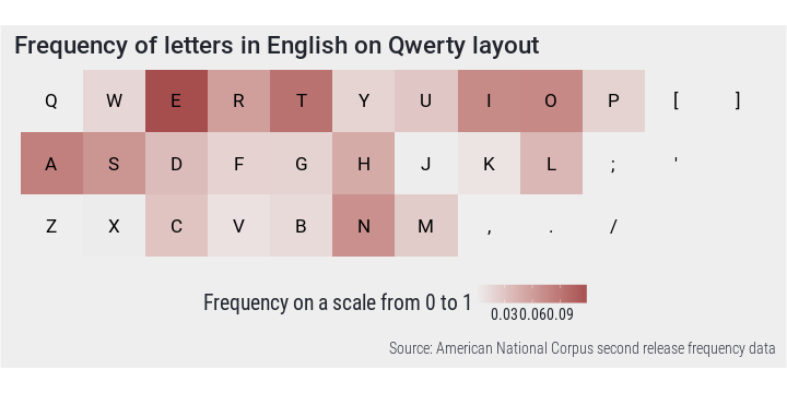
It’s evident from the plot that Dvorak puts more emphasis on the home row but it still lacks in this regard, especially with its location of R and L. Hand alternation is increased by having vowels on one side and most of consonants on the other.
PlotFreq(en.ag$val, dvo, en.ag$var, "Dvorak", clrs$dark[2])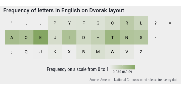
Colemak seems to be an improvement by placing all the most frequent letters on home row.
PlotFreq(en.ag$val, clm, en.ag$var, "Colemak", clrs$dark[3])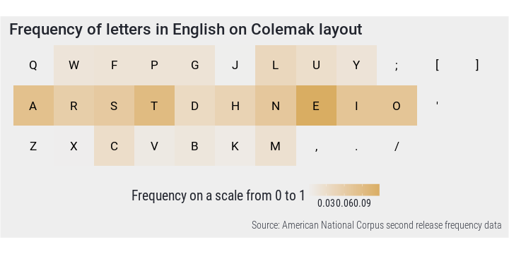
On the graph below, Qgmlwb does seem like the most optimal layout. Most frequent letters are on the home row and under the strongest fingers or near them. Placing consonants on one side and vowels on the other should result in improved alternation between hands.
PlotFreq(en.ag$val, qgm, en.ag$var, "Qgmlwb", clrs$dark[4])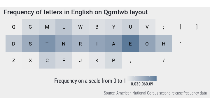
Share of letters typed on homerow
The code chunk below calculates the number of letters that can be typed on home row in each word for each layout. Note that there are likely more elegant ways of doing this than several nested apply functions. But this works, too.
hmr <-
  data.frame(word.sample,
             lapply(list(qwe, dvo, clm, qgm), function(x)
               sapply(
                 sapply(tolower(word.sample), function(y)
                   lapply(strsplit(y, ''), function(z)
                     ifelse(z %in% x[c(2, 5, 8, 11, 14, 17, 20, 23, 26, 29)], 1, 0))),
                 sum)), stringsAsFactors = F)
names(hmr) <- c('word', 'qwerty', 'dvorak', 'colemak', 'qgmlwb')

SampleRows(hmr, 10)
## word qwerty dvorak colemak qgmlwb
## 9862 my 0 0 0 0
## 52521 to 0 2 2 2
## 97454 to 0 2 2 2
## 50669 sit 1 3 3 3
## 16778 produced 2 5 5 5
## 13879 huh-uh 3 5 3 3
## 17218 this 2 4 4 4
## 47635 was 2 2 2 2
## 16788 of 1 1 1 1
## 56791 forced 2 3 4 4When using any of the alternative layouts, more than twice as many keystrokes are executed on home row as with Qwerty. There is little difference between the alternative layouts, however.
PlotBar(hmr, "Letters typed on homerow", "Letters typed on homerow / total number of letters")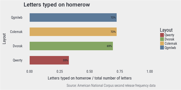
The density plot below illustrates the distribution of words by proportion of home row letters for each layout. In case of all layouts, there are many words that require half of keystrokes to be executed on home row. However, when using Qwerty many words are also typed without using home row at all, while the design of other layouts allows typing a large share of words only on homerow. Note that Colemak and Qgmlwb have the same letters on homerow which is why the line for Colemak is not visible here.
PlotDensity(hmr, "Letters typed on homerow by word", "Letters typed on homerow / all letters")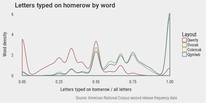
Hand alterations
Hand alteration here means typing consecutive letters with different hand fingers. This should speed up typing as it allows one hand to move to the next position while another hand is doing the key pressing. In order to determine the number of hand alternations in each word, we first assign l to each letter typed with a left hand finger and r to letters typed with a right hand finger. Then we calculate the number of different consecutive letters in each word in our sample.
alt <-
  data.frame(word.sample,
             lapply(list(qwe, dvo, clm, qgm), function(x) {
               sapply(unname(
                 lapply(
                   sapply(tolower(word.sample),
                          function(y) {lapply(strsplit(y, ''), function(z) {
                            ifelse(z %in% x[1:15], 'l',
                                   ifelse(z %in% x[16:36], 'r', '?'))
                          })
                            }),
                   function(q) rle(q)$lengths)), function(w) length(unlist(w)) - 1)
             }), stringsAsFactors = F)
names(alt) <- c('word', 'qwerty', 'dvorak', 'colemak', 'qgmlwb')

SampleRows(alt, 10)
## word qwerty dvorak colemak qgmlwb
## 54299 shakers 4 2 4 2
## 86495 man 2 2 2 2
## 46149 to 1 1 1 1
## 47912 the 2 1 1 1
## 17429 way 1 1 1 1
## 11639 were 0 3 3 3
## 38845 a 0 0 0 0
## 81624 important 3 5 5 5
## 71851 yet 1 1 1 1
## 85207 an 1 1 1 1On the bar chart below, the sum of all alterations is divided by the sum of all characters. It appears that Dvorak which was designed with this feature in mind, is the most successful in this respect with Qgmlwb being quite similar. When taking into account typing only single words, most of keystrokes on these layouts are followed by a press with another hand finger. This is not true for Colemak or Qwerty.
PlotBar(alt, "Alteration between hands", "Hand alterations / total number of keystrokes")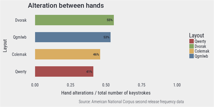
Looking at density chart, the previous finding is confirmed. Qwerty has the most words without any alterations, while most words fall on the right side of graph when typed on Dvorak. However, on all layouts it’s most common to change hands after every two letters, again not taking into account spaces between words.
PlotDensity(alt, "Alteration between hands by word", "Hand alterations / keystroke")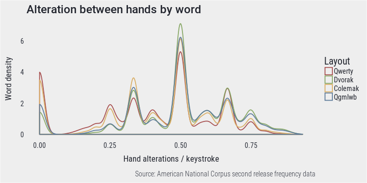
Inwards rolling motions
Inwards rolling motions are keystroke sequences that are executed from little finger towards index finger. For instance, on a Qwerty layout it’s convenient to type wear but read is not as natural. In order to evaluate the frequency of such movements, we replace each letter with it’s row number and then count certain patterns (rolling.motions) in each word. Here we consider sequences over multiple columns also as inwards rolling sequences (e.g. AS, AD, AF and AG on Qwerty layout).
rolling.motions <- c('12', '23', '34', '87', '98', '109',
                     '13', '24', '14', '97', '108', '107',
                     '15', '25', '35', '45', '106', '96', '86', '76')
CountMatches <- function(pat, vec) sapply(regmatches(vec, gregexpr(pat, vec)), length)
rol <-
  data.frame(word.sample,
             lapply(list(qwe, dvo, clm, qgm), function(w)
               unlist(lapply(
                 lapply(
                   lapply(
                     lapply(strsplit(word.sample, ''),
                            function(x) sapply(x, function(y) which(w == y, arr.ind = T)[2])),
                     function(q) paste(q, collapse = '')),
                   function(z) mapply(CountMatches, rolling.motions, z)),
                 sum))), stringsAsFactors = F)
names(rol) <- c('word', 'qwerty', 'dvorak', 'colemak', 'qgmlwb')

SampleRows(rol, 10)
## word qwerty dvorak colemak qgmlwb
## 74690 to 0 0 0 0
## 30290 'd 1 0 1 0
## 90038 was 1 0 1 0
## 17676 here 1 0 0 1
## 92214 was 1 0 1 0
## 78944 in 1 0 1 0
## 6816 we 1 0 0 0
## 2526 for 0 0 0 0
## 97775 it 0 0 0 0
## 65932 brothers 1 1 1 1Inwards rolling motions seem to be most frequent when using Qwerty but also Colemak layout where 16-17% of keystrokes are part of such movements This is expected in case of Colemak which was designed with this idea in mind. There seems to be a certain tradeoff between hand alterations and rolling motions since Dvorak and Qgmlwb seem to perform worse in this area.
PlotBar(rol, "Inward rolling sequences", "Inward rolling sequences / total number of keystrokes")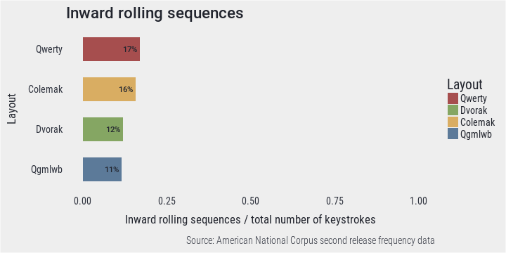
Word density suggests that layouts do not actually differ very much in respect to the typing gestures considered here. In a lot of words inward rolling sequences do not occur at all on any layout and there are very few words where most of keystrokes are part of such motion.
PlotDensity(rol, "Inward rolling sequences by word", "Inward rolling sequences / keystroke")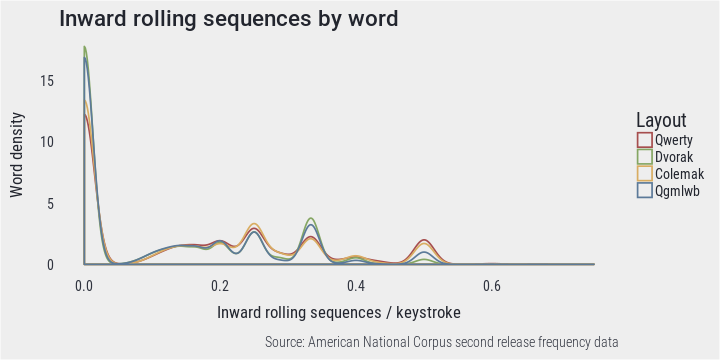
Conclusion
The previous knowledge of the advantages keyboard layouts gained some support with this simple evaluation. Qwerty is significantly less optimal than other layouts in terms of letter placement and home row usage. While Dvorak and Qgmlwb favor switching between hands, inwards rolling sequences are slightly more frequent when Qwerty and Colemak are used.