Propensity score matching with R

17 January 2018 - 19 mins read time
Tags: R Methods

In impact evaluations it is often necessary to measure the effect of a treatment, be it a support measure, training program or some other action. To make unbiased conclusions about the true effect, it is then necessary to take into account what would have happened without a treatment, i.e. evaluate the counterfactual situation. Subtracting the outcome of a control group from the result of treated observations allows us to do just that but it is crucial to control for selection bias. Impact evaluations are usually carried out retrospectively and many treatments permit random assignment of individuals into treatment and control groups. Thus, experimental research design (most prominently randomized controlled trials) can not be employed in such cases and we need to adopt non- or quasi-experimental methods. In the latter case, a pseudo control group is created so that it accurately reflects the counterfactual situation. Perhaps the most popular method for this purpose is propensity score matching (PSM), although the advantages of multivariate distance matching (MDM) (King and Nielsen 2016¹) must be noted. In case of PSM the propensity of each observation to be treated (i.e. propensity score) is assessed and then observations with close values of this assessment are compared. This allows us to compare observations where treatment can be the only source of differences in outcome, thus mitigating selection bias.

There are at least two R packages that help performing the matching, namely MatchIt and Matching. However, I felt like taking a more hands-on approach.

Data entry

In order to carry out PSM analysis we need a rather specific data set. Unfortunately, data that contains non-experimental treatment and control group as well as confounding variables predicting treatment and the outcome is rather hard to come by. Thus, we’ll be using data set provided by Lalonde (1986²) that includes the results of an employment and training program. This data set has previously been used by Sekhon (2011³) to demonstrate some functions related to PSM. The data is available for treatment and control group observations as separate tables. So we will load these tables and bind them into a data frame using only columns that are present in both tables. The last variables contain earnings of individuals in respective years.

# Download datasets if not present in working directory
for(i in c('nsw_treated.txt', 'cps_controls.txt')) {
  if (!file.exists(i)) {
    download.file(paste0('http://users.nber.org/~rdehejia/data/', i), i)
  }
}
rm(i)
# Load datasets
treated <- read.table('nsw_treated.txt',
                      col.names = c('treated', 'age', 'education', 'black', 'hispanic', 
                                    'married','nodegree', 're75', 're78'))
control <- read.table('cps_controls.txt',
                      col.names = c('treated', 'age', 'education', 'black', 'hispanic', 
                                    'married','nodegree', 're74', 're75', 're78'))
lalonde <- rbind(treated[intersect(colnames(treated), colnames(control))],
                 control[intersect(colnames(treated), colnames(control))])
head(lalonde)

##   treated age education black hispanic married nodegree re75       re78
## 1       1  37        11     1        0       1        1    0  9930.0460
## 2       1  22         9     0        1       0        1    0  3595.8940
## 3       1  30        12     1        0       0        0    0 24909.4500
## 4       1  27        11     1        0       0        1    0  7506.1460
## 5       1  33         8     1        0       0        1    0   289.7899
## 6       1  22         9     1        0       0        1    0  4056.4940

The problem

We use by to get the mean of different variables separately for treated and other individuals.

by(lalonde, lalonde$treated, colMeans)

## lalonde$treated: 0
##      treated          age    education        black     hispanic 
## 0.000000e+00 3.322524e+01 1.202751e+01 7.353677e-02 7.203602e-02 
##      married     nodegree         re75         re78 
## 7.117309e-01 2.958354e-01 1.365080e+04 1.484666e+04 
## -------------------------------------------------------- 
## lalonde$treated: 1
##      treated          age    education        black     hispanic 
## 1.000000e+00 2.462626e+01 1.038047e+01 8.013468e-01 9.427609e-02 
##      married     nodegree         re75         re78 
## 1.683502e-01 7.306397e-01 3.066098e+03 5.976352e+03

It is evident that our initial control group is unbalanced since the distribution of the characteristics of individuals is very different. The mean change in earnings for treated individuals between 1975 and 1978 is 2910. For others it is 1196. When adopting a “naive” approach we would assume that treatment increased mean earnings by the difference between the two values, i.e. 1714. As treated individuals might have had a higher increase even without treatment, we would thus overestimate the effect of treatment by considering all of the individuals. It is thus necessary to create a balanced pseudo control group in order to simulate the counterfactual situation.

Building propensity score model

Here we would like to assess the effect of treatment on earnings in 1978. We assume that age, years in education, race, marital status, academic degree and earnings in 1975 have an effect on both. So these need to be considered as confounding variables and will be used to calculate the propensity score.

Since treatment status is indicated as a binary (dummy) variable, we will fit a logistic regression model on the data. Then we perform a stepwise regression that seeks to minimize the value of Akaike Information Criterion (AIC).

prop.model <- glm(treated ~ age + education + black + hispanic + married + nodegree + re75, 
                  data = lalonde, family = binomial(link = "logit"))
step(prop.model)

## Start:  AIC=1546.88
## treated ~ age + education + black + hispanic + married + nodegree + 
##     re75
## 
##             Df Deviance    AIC
## <none>           1530.9 1546.9
## - education  1   1533.6 1547.6
## - age        1   1538.5 1552.5
## - nodegree   1   1568.4 1582.4
## - married    1   1577.0 1591.0
## - hispanic   1   1585.7 1599.7
## - re75       1   1617.7 1631.7
## - black      1   2271.7 2285.7

## 
## Call:  glm(formula = treated ~ age + education + black + hispanic + 
##     married + nodegree + re75, family = binomial(link = "logit"), 
##     data = lalonde)
## 
## Coefficients:
## (Intercept)          age    education        black     hispanic  
##  -5.3562180   -0.0227897    0.0641759    4.1588862    2.1743388  
##     married     nodegree         re75  
##  -1.2394148    1.2704833   -0.0001162  
## 
## Degrees of Freedom: 16288 Total (i.e. Null);  16281 Residual
## Null Deviance:	    2967 
## Residual Deviance: 1531 	AIC: 1547

According to AIC values, all of the variables improve the quality of the model.

Next, we examine coefficients.

summary(prop.model)

## 
## Call:
## glm(formula = treated ~ age + education + black + hispanic + 
##     married + nodegree + re75, family = binomial(link = "logit"), 
##     data = lalonde)
## 
## Deviance Residuals: 
##     Min       1Q   Median       3Q      Max  
## -1.3476  -0.0850  -0.0359  -0.0172   3.8175  
## 
## Coefficients:
##               Estimate Std. Error z value Pr(>|z|)    
## (Intercept) -5.356e+00  6.403e-01  -8.366  < 2e-16 ***
## age         -2.279e-02  8.470e-03  -2.691  0.00713 ** 
## education    6.418e-02  3.926e-02   1.635  0.10214    
## black        4.159e+00  2.009e-01  20.704  < 2e-16 ***
## hispanic     2.174e+00  2.704e-01   8.041 8.92e-16 ***
## married     -1.239e+00  1.904e-01  -6.511 7.45e-11 ***
## nodegree     1.270e+00  2.123e-01   5.984 2.18e-09 ***
## re75        -1.162e-04  1.404e-05  -8.278  < 2e-16 ***
## ---
## Signif. codes:  0 '***' 0.001 '**' 0.01 '*' 0.05 '.' 0.1 ' ' 1
## 
## (Dispersion parameter for binomial family taken to be 1)
## 
##     Null deviance: 2967.2  on 16288  degrees of freedom
## Residual deviance: 1530.9  on 16281  degrees of freedom
## AIC: 1546.9
## 
## Number of Fisher Scoring iterations: 9

prop.model <- glm(treated ~ age + black + hispanic + married + nodegree + re75, 
                  data = lalonde, family = binomial(link = "logit"))

The coefficient of education is not significantly different from zero, so we updated our model not to include it.

The dependent variable in logistic regression is binary and we can adjust the predicted values to describe binary outcome, too. Thus, we can draw a classification table that illustrates how well the model classifies the observations, taking the mean of fitted values as the threshold for predicting treatment.

table(prop.model$fitted.values > mean(prop.model$fitted.values), 
      lalonde$treated, dnn = c("Predicted", "True"))

##          True
## Predicted     0     1
##     FALSE 14309    33
##     TRUE   1683   264

The classification table indicates that the proportion of correctly classified treated observations is 1.

We also calculate a few other statistics that help us evaluate logistic regression model.

# McFadden's pseudo R-squared value of the model
1 - (prop.model$deviance/prop.model$null.deviance)

## [1] 0.4831533

# Test the model against a null model
pchisq(prop.model$null.deviance - prop.model$deviance, 
       prop.model$df.null - prop.model$df.residual, lower.tail = FALSE)

## [1] 1.266532e-306

According to McFadden (1978⁴), the value of McFadden’s pseudo-R between 0.2 and 0.4 indicates an excellent model fit. The value we obtained is even higher. We can also reject the null hypothesis that all the coefficients in the model equal zero.

This model performs well enough on our data to use the fitted values of the dependent variable as propensity score values for each individual.

Creating pseudo control group

Next we create a new variable and assign it propensity scores from the model. We can again use by to examine summary statistics of propensity scores separately for treated and other individuals.

lalonde$propensity <- c(prop.model$fitted.values, use.names = F)
by(lalonde$propensity, lalonde$treated, summary)

## lalonde$treated: 0
##      Min.   1st Qu.    Median      Mean   3rd Qu.      Max. 
## 0.0000441 0.0001544 0.0006743 0.0129976 0.0038139 0.5820945 
## -------------------------------------------------------- 
## lalonde$treated: 1
##      Min.   1st Qu.    Median      Mean   3rd Qu.      Max. 
## 0.0007684 0.1232701 0.2850716 0.3001407 0.5037444 0.5756670

The comparison of two groups can also be plotted and adding some jitter gives a better overview. A better plot type for this kind of comparison might be a density plot, but plotting points is more intuitive.

plot(lalonde$propensity, jitter(lalonde$treated), 
     xlab = "Propensity score", ylab = "Treatment status")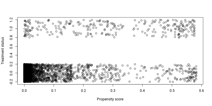

As anticipated, the probability of treated observations to be treated is substantially higher since a great majority of non-treated individuals have a propensity score close to 0. This is an indication that the groups are unbalanced and it is necessary to create a pseudo control group for a more fair comparison.

There are various matching techniques that can be implemented to select appropriate individuals for control group, e.g. nearest-neighbour, caliper, radius or kernel matching. Here we will use the first approach due to its simplicity. First we create a function that (1) takes the propensity score of each treated individual, (2) finds the row of a control group individual that has the most similar propensity score value and (3) returns a logical vector indicating control group members. Thus, the matching is done with replacements, i.e. one control group individual may be matched to more than one treated individual.

Match <- function(data, treated.var, score.var) {
  # Convert treated.var into logical
  data[, treated.var] <- as.logical(data[, treated.var])
  # Find closest non-treated score to each treated score
  vec <- sapply(data[data[, treated.var], score.var], 
                function(x) which.min(abs(x - data[!data[, treated.var], score.var]))) 
  # Return a logical vector indicating rows of control group
  return(rownames(data) %in% rownames(data[!data[, treated.var], ])[unique(vec)])
}

Now we apply this function to our data frame.

lalonde$control <- Match(lalonde, 'treated', 'propensity')

When plotting the propensity scores of the pseudo control group we obtained by implementing our matching algorithm, it is evident that the distribution of scores is much more similar now.

with(lalonde[lalonde$treated == 1 | lalonde$control, ], 
             plot(propensity, jitter(treated), 
                  xlab = "Propensity score", ylab = "Treatment status"))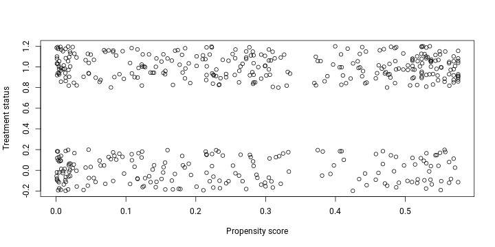

Balancing

In order to achieve a meaningful comparison of treatment and control group it is necessary that the groups are similar in terms of all the factors that being treated or not depends on. In other words, the groups need to be balanced. In our case, we need to have the groups balanced according to the independent (confounding) variables that we included in the model for predicting treatment. One simple way to check the balance is by comparing the mean values of treatment, control and pseudo control groups. Sometimes hypothesis testing is used to confirm the lack of difference in distribution or some particular statistic of values but it is usually not recommended.

# Set confounding variables from propensity model
confounding <- names(coefficients(prop.model))[-1]
# Generate data frame with mean values of confounding variables by group
balance <- data.frame(control = sapply(lalonde[lalonde$treated == 0, confounding], mean),
                      treated = sapply(lalonde[lalonde$treated == 1, confounding], mean),
                      pseudo.control = sapply(lalonde[lalonde$control, confounding], mean))

# Format and print the comparison
format(balance, digits = 2, scientific = F)

##            control  treated pseudo.control
## age         33.225   24.626          27.69
## black        0.074    0.801           0.73
## hispanic     0.072    0.094           0.11
## married      0.712    0.168           0.23
## nodegree     0.296    0.731           0.66
## re75     13650.803 3066.098        3608.61

We can see that when deciding by the mean values for several variables the balance has become better. At this point we might want to go back and adjust the propensity model or matching algorithm but here we are just providing an example. It is important to note that the confounding effect may be more significant for some variables so it is not always necessary to have the groups balanced across all of them.

Estimating the impact of treatment using control group

Here we apply a differences-in-differences approach which means that we don’t only compare the differences between groups but also time. Adding another dimension by comparing change rather than merely the difference of values after treatment allows us to use more information and thus gives a more accurate estimation of the effect of treatment. Let us calculate the change of mean earnings for all three groups.

# Change in income for treated individuals
change.treated <- lalonde$re78[lalonde$treated == 1] - lalonde$re75[lalonde$treated == 1]
mean(change.treated)

## [1] 2910.254

# Change in income for control group individuals 
change.control <- lalonde$re78[lalonde$treated == 0] - lalonde$re75[lalonde$treated == 0]
mean(change.control)

## [1] 1195.856

# Change in income for individuals in pseudo control group
change.pseudo <- lalonde$re78[lalonde$control] - lalonde$re75[lalonde$control]
mean(change.pseudo)

## [1] 3067.741

As previously explained, if we considered the original control group to reflect the counterfactual situation, we could claim that earnings increased by 1714 due to treatment. That seems like an overestimation. When we instead use the mean change in earnings of pseudo control group, we conclude that earnings changed by -157. So treatment actually had a slight negative effect on earnings according to means of changes. These results might be better illustrated by t-tests.

# Test of difference in means of treated and control group
t.test(change.treated, change.control)

## 
## 	Welch Two Sample t-test
## 
## data:  change.treated and change.control
## t = 3.5225, df = 305.52, p-value = 0.0004928
## alternative hypothesis: true difference in means is not equal to 0
## 95 percent confidence interval:
##   756.6813 2672.1138
## sample estimates:
## mean of x mean of y 
##  2910.254  1195.856

# Test of difference in means of treated and pseudo control group
t.test(change.treated, change.pseudo)

## 
## 	Welch Two Sample t-test
## 
## data:  change.treated and change.pseudo
## t = -0.24036, df = 483.79, p-value = 0.8102
## alternative hypothesis: true difference in means is not equal to 0
## 95 percent confidence interval:
##  -1444.912  1129.938
## sample estimates:
## mean of x mean of y 
##  2910.254  3067.741

The p-values of the two t-tests also indicate that previously we could have attributed a substantial increase in mean earnings to treatment. After implementing PSM we were unable to demonstrate the mean effect of treatment to be statistically significant and thus we conclude that treatment had no impact on earnings.

References