class: center, middle, inverse, title-slide # Simple linear regression ## Research methods ### Jüri Lillemets ### 2021-12-01 --- class: center middle clean # How can we model a relationship? --- class: center middle inverse # Ordinary least squares --- ## Example problem Suppose we have data on the "Weight gain calves in a feedlot, given three different diets." | animal| herd|diet | initialwt| finalwt| |------:|----:|:----|---------:|-------:| | 1| 9|Low | 575| 826| | 2| 9|Low | 605| 816| | 3| 9|Low | 640| 902| - `animal`, animal ID - `herd`, herd ID - `diet`, diet: Low, Medium, High - `initialwt`, initial weight - `finalwt`, slaughter weight --- .pull-left[ Let's see initial and slaughter weight of calves. <!-- --> ] -- .pull-right[ Does initial weight have an effect on final weight? How much of final weight depends on initial weight? How much does final weight increase when initial weight increases? What could be the final weight when initial weight is e.g. 700? Can we quantify this relationship? ] ??? Draw possible lines. --- We can model this by estimating a regression model! <!-- --> --- ## Model specification Regression models represent how one or more more predictor variables ( `\(x_k\)` ) have an effect on a response variable ( `\(y\)` ): `$$\hat{y} = \sum^K_{k=1}x_k.$$` The most simple regression model has only one predictor, which is why it is called "simple linear regression" (SLS). --- An *single least squares* (*SLS*) model is mathematically expressed as follows: `$$\hat{y} = \beta_0 + \beta_1 x + \varepsilon,$$` where - `\(\hat{y}\)` is dependent or explained variable, **response** or regressand, - `\(\beta_0\)` is the intercept or constant, - `\(\beta_1\)` is a coefficient of `\(x\)`, - `\(x\)` is independent or explanatory variable, **predictor** or regressor, and - `\(\varepsilon\)` is the model error or residual. ??? The values of `\(x\)` and `\(y\)` come from our data, whereas the `\(\beta_1\)` coefficients need to be calculated from this data. The `\(\varepsilon\)` is estimated using both, the `\(\beta_1\)` coefficients and data. --- In our example the formula can be expressed as `$$\text{finalwt} = \beta_0 + \beta_1 \text{initialwt} + \varepsilon_i.$$` For first 3 observations in our data this model can be expressed as `$$\begin{matrix} 826 \\ 816 \\ 902 \end{matrix} = \beta_0 + \beta_1 \times \begin{matrix} 575 \\ 605 \\ 640 \end{matrix} + \begin{matrix} \varepsilon_1 \\ \varepsilon_2 \\ \varepsilon_3 \end{matrix}.$$` -- Residuals, `\(\varepsilon_i\)` can be calculated after we have found `\(\beta_0\)` and `\(\beta_1\)`. But how do we find the `\(\beta_0\)` and `\(\beta_1\)`? --- ## Calculation of an SLS model The idea is to minimize squared residuals, thus the name "least squares". For `\(Y = \beta_0 + \beta_1 x + \varepsilon\)` we can do this as follows: `\(\hat{\beta_1} = \frac{Cov[x,y]} {Var[x]} = \frac{\sum{x_{i} y_{i}} - \frac{1}{n} \sum{x_{i}}\sum{y_{i}}}{\sum{x_{i}^{2}} - \frac{1}{n} (\sum{x_{i}})^{2}}\)`, `\(\hat{\beta_0} = \overline{y} - \hat\beta_1 \overline{x}.\)` -- In our example `\(x\)` would be the vector of initial weights. ``` ## [1] 575 605 640 600 610 575 730 670 690 685 690 670 755 655 725 750 705 785 685 ## [20] 655 750 715 785 795 640 680 620 765 750 645 730 795 605 570 730 670 700 665 ## [39] 635 700 715 675 770 800 685 715 865 845 705 725 840 755 725 770 755 530 680 ## [58] 605 665 765 720 780 675 705 755 755 750 ``` And `\(x\)` would be the vector of final weights. ``` ## [1] 826 816 902 931 854 960 1104 922 1046 1027 1018 864 1008 979 1085 ## [16] 1037 1123 1171 1018 1027 1152 1142 1104 1152 941 979 931 1133 989 970 ## [31] 1162 1248 874 854 1046 1056 1037 874 874 998 960 979 1056 1133 1027 ## [46] 1037 1219 998 1037 1075 1190 1104 883 1123 1056 883 1018 874 970 1114 ## [61] 1018 1152 1056 1066 1104 1114 1008 ``` --- For a model `\(y = \beta_1 x + \varepsilon\)` we can simply use matrix algebra on values of `\(x\)` and `\(y\)`: `$$\hat{\beta_1} = (X^\prime X)^{-1} X^\prime Y$$` -- In our example problem `\(X\)` would be the column vector of initial weights. | | |---:| | 575| | 605| | 640| And `\(Y\)` would be the column vector of final weights. | | |---:| | 826| | 816| | 902| --- > Why is one variable dependent and other(s) independent? <!-- --> --- Because we try to minimize error in response variable. -- <!-- --> Using response to predict predictor would give us a different regression line! --- class: center middle inverse # Elements of a regression model --- ## Intercept In the equation `\(\hat{y} = \beta_0 + \beta_1 x + \varepsilon,\)` intercept is the `\(\beta_0\)`. Intercept is sometimes also called *constant*. It is the value of `\(y\)` where regression line crosses the y-axis, so intercept is the value of `\(y\)` when `\(x\)` is zero ( `\(y|x=0\)` ). Intercept is theoretically irrelevant when the range of our observed values of `\(x\)` does not cover 0. --- Intercept is the value of `\(y\)` where regression line crosses the y-axis. 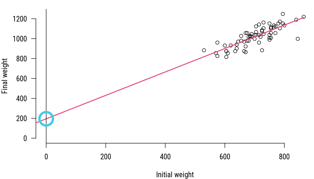<!-- --> -- > Does the intercept make sense in this example? --- In our example final weight is 195 if initial weight is 0. Intercept is not always meaningful. ``` ## ## Call: ## lm(formula = finalwt ~ initialwt, data = calves) ## ## Residuals: ## Min 1Q Median 3Q Max ## -190.66 -32.48 11.59 34.30 118.13 ## ## Coefficients: ## Estimate Std. Error t value Pr(>|t|) ## (Intercept) 195.1352 76.5219 2.55 0.0131 * ## initialwt 1.1758 0.1083 10.86 3.02e-16 *** ## --- ## Signif. codes: 0 '***' 0.001 '**' 0.01 '*' 0.05 '.' 0.1 ' ' 1 ## ## Residual standard error: 61.27 on 65 degrees of freedom ## Multiple R-squared: 0.6447, Adjusted R-squared: 0.6392 ## F-statistic: 117.9 on 1 and 65 DF, p-value: 3.017e-16 ``` --- Intercept should not be interpreted when it requires extrapoliation of observed data.  .footnote[Source: Xkcd. Extrapolating] --- ## Coefficient(s) In the equation `\(\hat{y} = \beta_0 + \beta_1 x + \varepsilon,\)` coefficients are the `\(\beta_1\)`. Coefficient(s) indicate by how many units `\(y\)` increases when `\(x\)` increases by one unit. --- By how many units final weight increase when initial weight increases by one unit. 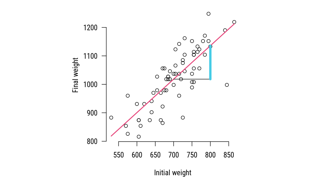<!-- --> -- > What could be the value of `\(\beta_1\)` in this example? --- In our example every kg of initial weight increases final weight by 1.176 kg (on the plot `\(\times 100\)`). ``` ## ## Call: ## lm(formula = finalwt ~ initialwt, data = calves) ## ## Residuals: ## Min 1Q Median 3Q Max ## -190.66 -32.48 11.59 34.30 118.13 ## ## Coefficients: ## Estimate Std. Error t value Pr(>|t|) ## (Intercept) 195.1352 76.5219 2.55 0.0131 * ## initialwt 1.1758 0.1083 10.86 3.02e-16 *** ## --- ## Signif. codes: 0 '***' 0.001 '**' 0.01 '*' 0.05 '.' 0.1 ' ' 1 ## ## Residual standard error: 61.27 on 65 degrees of freedom ## Multiple R-squared: 0.6447, Adjusted R-squared: 0.6392 ## F-statistic: 117.9 on 1 and 65 DF, p-value: 3.017e-16 ``` --- The interpretation of `\(\beta_1\)` is different if `\(x\)` is a categorical variable. Suppose that a categorical variable called `diet` has the following levels: *Low, High, Medium*. When we use it as a predictor then the first level (*Low*) is considered as the base level. All other factor values are compared against the base level. --- When we have `diet` as a predictor instead of `initialwt`, then we have the following model: `$$finalwt_{i} = 1019.406 + 12.01dietMedium_{i} + 1.898dietHigh_{i} + \varepsilon_{i}.$$` When `diet` is Low, then final weight is 1019.406. When `diet` is High, then final weight is higher by 12.01 units compared to when `diet` is Low 1031.417. -- > When diet is Medium, how much higher is final weight compared to when diet is Low? --- ### Statistical significance of coefficients We usually estimate models on a sample and wish to make generalizations or inferences about population. Coefficients are only relevant if their difference from 0 is statistically significant. If a coefficient is not statistically significant, then we would conclude that the predictor has no effect on the response. -- The idea of testing statistical significance of a coefficient is equivalent to a t-test! --- It is always necessary to test whether or not coefficients are different from 0. This is done by calculating t-statistic from coefficient and standard error. ``` ## ## Call: ## lm(formula = finalwt ~ initialwt, data = calves) ## ## Residuals: ## Min 1Q Median 3Q Max ## -190.66 -32.48 11.59 34.30 118.13 ## ## Coefficients: ## Estimate Std. Error t value Pr(>|t|) ## (Intercept) 195.1352 76.5219 2.55 0.0131 * ## initialwt 1.1758 0.1083 10.86 3.02e-16 *** ## --- ## Signif. codes: 0 '***' 0.001 '**' 0.01 '*' 0.05 '.' 0.1 ' ' 1 ## ## Residual standard error: 61.27 on 65 degrees of freedom ## Multiple R-squared: 0.6447, Adjusted R-squared: 0.6392 ## F-statistic: 117.9 on 1 and 65 DF, p-value: 3.017e-16 ``` -- > Is the coefficient statistically significant? Is there an effect? --- ## Fitted values In the equation `\(\hat{y} = \beta_0 + \beta_1 x + \varepsilon,\)` fitted values are the `\(\hat{y}\)`, i.e. estimations of `\(y\)`. These are the estimated values of response ( `\(\hat{y}\)` ) that are calculated by applying the model for `\(x\)` of every observation in the data. In other words, fitted values are model estimations or *predictions* of `\(y\)` for each observation. --- Fitted values express response according to model. 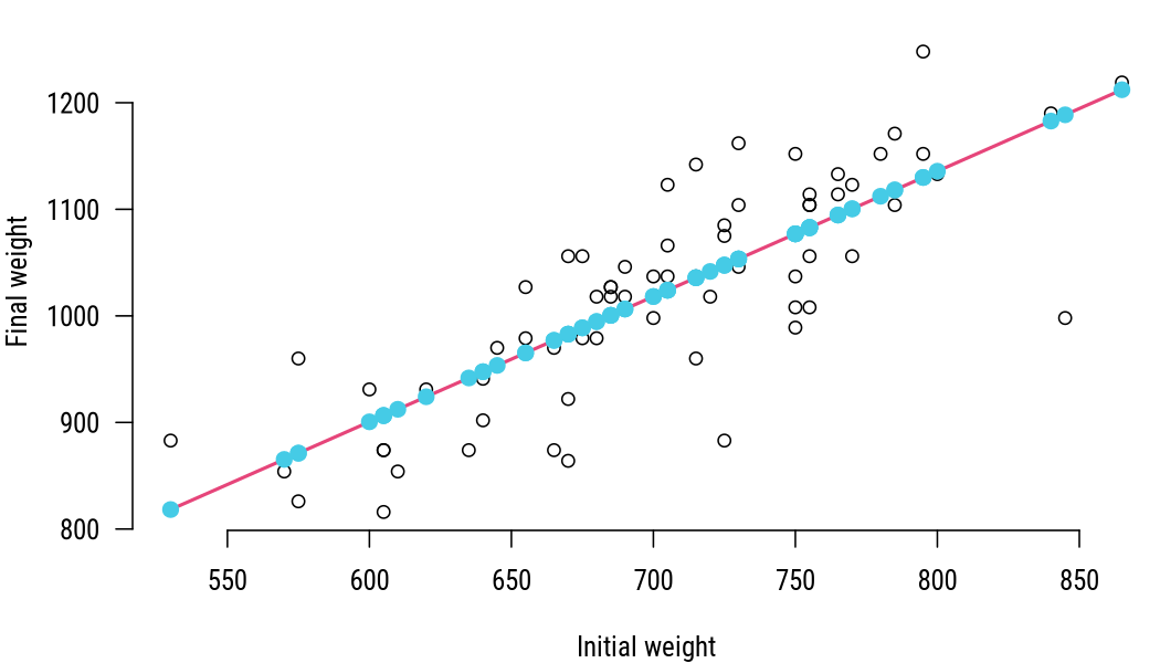<!-- --> -- > What will be the approximate final weight for a calf whose initial weight is 700? --- ### Predictions After we have estimated the `\(\beta_0\)` and `\(\beta_1\)`, we have a model. We can use this model to calculate fitted values `\(\hat{y}\)` for each value of `\(x\)` as follows: `\(\hat{y} = \beta_0 + \beta_1 x\)`. `$$\text{finalwt} = \beta_0 + \beta_1 \text{initialwt} + \varepsilon$$` Because we find fitted values assuming no errors, the residual is zero and can thus be ignored. -- What is the exact final weight if initial weight is 700? `$$195.1352374 + 1.1757679 \times 700 = 1018.1727372$$` --- ## Residuals In the equation `\(\hat{y} = \beta_0 + \beta_1 x + \varepsilon,\)` residuals are the `\(\varepsilon\)`. Residuals are the differences of observed `\(y\)` and fitted values of `\(y\)`. Residuals are essentially errors that our model makes. We can find residuals for each observation after we have estimated `\(\beta_0\)` and `\(\beta_1\)` using values of `\(x\)` and `\(y\)` as follows: `\(\varepsilon = y - \beta_0 - \beta_1 x\)`. --- We use residuals to evaluate how well model fits data. > Suppose that a model has relatively large residuals. Does the model have a good fit? -- Large residuals would mean that fitted values are different from observed values, which indicates that model does not fit data well. --- Residuals are differences between of observed and fitted values of response. 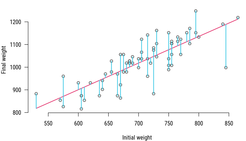<!-- --> --- ## The `\(R^2\)` This is a way to measure *goodness of fit* of a model, i.e. how well model fits data. It is sometimes called *coefficient of determination*. `\(R^2\)` expresses the part of variation in response variable that is explained by a model. More precisely, `\(R^2\)` measures how much better is model at explaining the variance of `\(y\)` compared to how well just the **mean** of `\(y\)` (i.e. `\(E(y)\)`) explains variance of `\(y\)`. --- The `\(R^2\)` is equal to squared value of Pearson's `\(r\)` between observed values of `\(y\)` and fitted values `\(\hat{y}\)`. If fitted values of `\(y\)` are similar to observed values of `\(y\)`, there is a high correlation and Pearson's `\(r\)` and thus also `\(R^2\)` are high. --- How do find the variation in `\(y\)` that a model explains? $$R^{2} = \frac{ESS}{TSS} = 1 - \frac{RSS}{TSS}, $$ where the elements are defined a follows: - **e**xplained sum of squares, `\(ESS\)`; `\(\sum_{i = 1}^{n} (\hat{y}_{i} - \bar{y})^2\)` - **r**esidual sum of squares, `\(RSS\)`; `\(\sum_{i = 1}^{n} (y_{i} - \hat{y}_{i})^2\)` - **t**otal sum of squares, `\(TSS\)`; `\(\sum_{i = 1}^{n} (y_{i} - \bar{y})^2.\)` --- `\(R^2\)` expresses how much better is model at explaining the variance of `\(y\)` compared to just the mean? 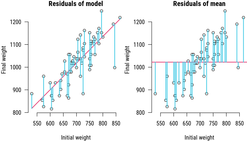<!-- --> ??? This is simplification, we're actually using squared distances. --- It's always a good idea to plot observed data. 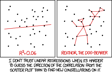 .footnote[Source: Xkcd. Linear regression] --- ## The adjusted- `\(R^2\)` The more predictors we add, the more the model explains variance of `\(y\)`. So `\(R^2\)` can be inflated just by adding more predictors to the model even if the predictors are not very meaningful. -- To penalize a model for the number of predictors ( `\(k\)` ) while considering the number of observations ( `\(n\)` ), the adjusted `\(R^{2}\)` can also be used, particularly for model comparison: `$$\overline{R^{2}} = 1 - \frac{RSS/(n-k)}{TSS/(n-1)}$$` --- Most software calculates `\(R^2\)` with the model and prints it with model summary. ``` ## ## Call: ## lm(formula = finalwt ~ initialwt, data = calves) ## ## Residuals: ## Min 1Q Median 3Q Max ## -190.66 -32.48 11.59 34.30 118.13 ## ## Coefficients: ## Estimate Std. Error t value Pr(>|t|) ## (Intercept) 195.1352 76.5219 2.55 0.0131 * ## initialwt 1.1758 0.1083 10.86 3.02e-16 *** ## --- ## Signif. codes: 0 '***' 0.001 '**' 0.01 '*' 0.05 '.' 0.1 ' ' 1 ## ## Residual standard error: 61.27 on 65 degrees of freedom ## Multiple R-squared: 0.6447, Adjusted R-squared: 0.6392 ## F-statistic: 117.9 on 1 and 65 DF, p-value: 3.017e-16 ``` --- How are the parameters related to the formula? `$$finalwt_{i} = 195 + 1.176 * initialwt_{i} + \varepsilon_{i}$$` How do the values of first observation fit into the model? | | Value| |:---------|----------:| |initialwt | 575.000000| |finalwt | 826.000000| |beta_0 | 195.135237| |beta_1 | 1.175768| |residual | -45.201755| |fitted | 871.201755| --- class: center middle inverse # Assumptions and diagnostics --- ## Residuals are normally distributed 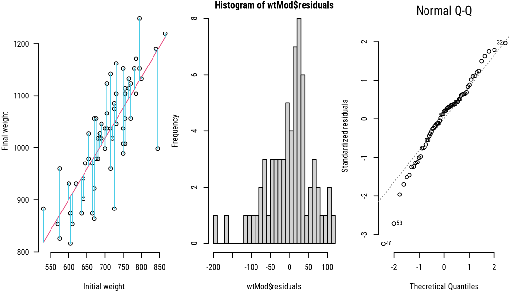<!-- --> --- ## Residuals have equal variance 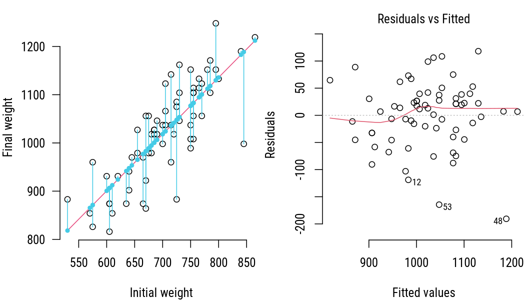<!-- --> -- Here the we have equal variance, e.g. **homo**scedasticity. ??? Variance of residuals does not depend on the value of `\(x\)`. --- Example of **hetero**scedasticity. Here higher values have higher variance than lower. <!-- --> --- ## Gauss-Markov assumptions Linear model must fulfill the following conditions according to Gauss–Markov theorem: - linear in parameters `\(Y = \beta_0 + \beta_1 x + \varepsilon\)` - expected error is zero `\(E(\varepsilon) = 0\)` - homoscedasticity `\(var(\varepsilon) = E(\varepsilon^{2})\)` - no autocorrelation `\(cov(\varepsilon_{i}, \varepsilon_{j}) = 0, i \neq j\)` - independence of predictor(s) and residuals `\(cov(x,\varepsilon) = 0\)` -- If these assumptions are met, then the model is the *best linear unbiased estimator* (BLUE). --- class: center middle inverse # Practical application --- Use the data set `HousePrices`. Estimate sale price of a house (`price`) using lot size of a property (`lotsize`) as a predictor. > Are residuals normally distributed? > Do residuals have equal variance? > Does the size of a property have an effect on sale price? -- > How exactly does the size of a property influence sale price? --- Use the same data set. Estimate sale price of a house (`price`) using the presence of air conditioning (`aircon`) as a predictor. > Are residuals normally distributed? > Do residuals have equal variance? > Does the presence of air conditioning have an effect on sale price? > How exactly does the presence of air conditioning influence sale price? -- A regression model with only categorical predictor(s) is actually equivalent to a t-test or ANOVA. --- class: inverse ???